Listing all Hamiltonian cycles of the graph

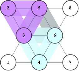
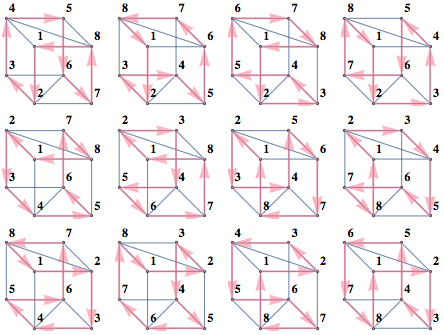
You can encode Hamiltonian cycle problem into SAT. It's more complicated than independent sets in previous post, but it can be done by assigning number to each vertex indicating its position in Hamiltonian cycle, constraining chosen edges to be consistent with vertex numbering, and using SatisfiabilityInstances to find all satisfying assignments

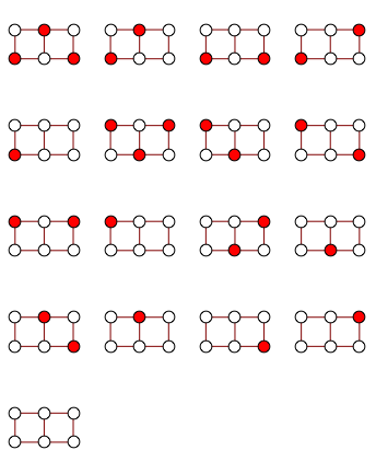
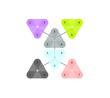
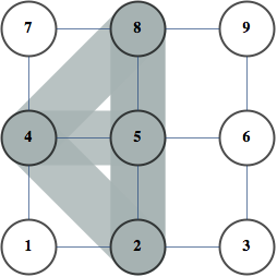
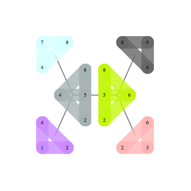
Here are the 12 cycles produced this way for BislitCube


Here are the constraints that were used

• Every vertex has one incoming and one outgoing edge
  
• Cycles of length 2 are forbidden
  
• Every vertex is assigned one number
  
• First vertex is assigned number 1
  
• Presence of edge i,j implies number of number(j)=number(i)+1 and the converse
  

Smaller number of constraints can be used, but I found that increasing constraints makes SAT solver faster.

For these Graph Theory -> SAT encoding tasks, I find it helpful to have "formula"/ "vars" variables, and "decodeInstance"/"drawInstance" functions that so I can do something like this

sats = SatisfiabilityInstances[formula, vars, 20];
drawInstance /@ sats
decodeInstance /@ sats

decodeInstance turns variable assignment into readable/easy to process format, whereas drawInstance visualizes the instance as in pictures above.

Below is the notebook used to generate this diagram. It also has a helper .m file to draw a grid of all graphs with given set of properties. For instance, to show all graphs in GraphData that have 12 vertices, are Planar, Connected but are not Trees and fit in a 6x6 grid you would do

Needs["Bulatov`showGraphs`"];
showGraphs[12, "Connected", ! "Tree", "Planar", gridSize -> 6]

Name of graph shows up in Tooltip

Notebook+package

Using SAT solver to find independent sets

Here's a simple graph and all of its independent vertex sets



You can use SatisfiabilityInstances to get them as follows

gg = GridGraph[{2, 3}];
edge2clause[e_] := ! (e[[1]] && e[[2]]);
clauses = edge2clause /@ EdgeList[gg];
formula = And @@ clauses;
vars = VertexList[gg];
instances = SatisfiabilityInstances[formula, vars, 1000];
independentSets = Extract[vars, Position[#, True]] & /@ instances

Notebook

Counters in SAT

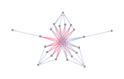
Here's a visualization of a SAT formula of a BooleanCountingFunction. Four circles in the middle are the variables of interest. Five circles on the periphery are variables encoding the number of true assignments of the four circles in the middle. Squares are clauses, and color of the edge indicates whether the variable is negated in that clause. You can see from the color that rightmost circle represents "all variables are true" and leftmost circle represents "all variables are false".



Notebook

Tree decomposition package

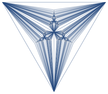
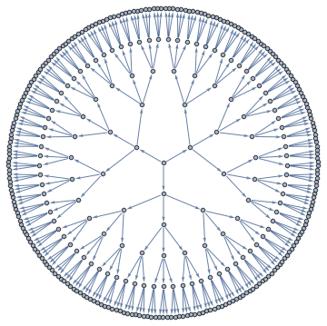
A tree decomposition is a representation of a complete set of vertex separators of a graph. For instance, here's an Apollonian Network and its tree decomposition.




Decomposition above shows off 121 vertex separators of size 4, represented as non-leaf nodes, each separating graph into 3 parts, and 363 vertex separators of size 3, represented as edges, each separating the graph into 2 parts.

I put the tree decomposition code in a package. Unzip the file into any folder, and execute cells in treeDecomposition-usage.nb for the decomposition above. It takes 2 minutes for 367 vertex Apollonian network above. Graphs with around hundred vertices should take a few seconds.

Generally, to do a visualization like above, you'd do the following

<< Bulatov`treeDecomposition`;
g = GraphData[{"Apollonian", 5}];
{nodes, edges} = findTreeDecomposition[g];
GraphPlot[Rule @@@ edges]

Tree decomposition package

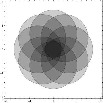
Coloring overlapping circles

Take some overlapping circles

nc = 8;
ineqs = Table[(x - 2/3 Cos[i 2 Pi/nc])^2 + (y - 
        2/3 Sin[i 2 Pi/nc])^2 < 1, {i, 0, nc - 1}];
Show[Table[
  RegionPlot[ineqs[[k]], {x, -2, 2}, {y, -2, 2}, PlotPoints -> 35, 
   PlotStyle -> Opacity[.2]], {k, 1, nc}]]

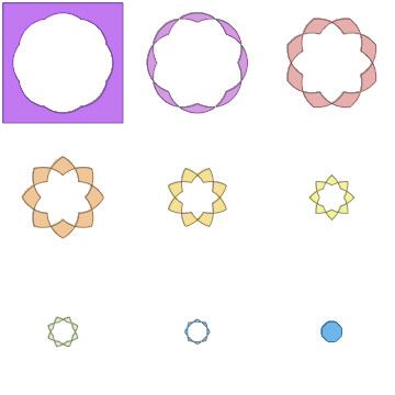
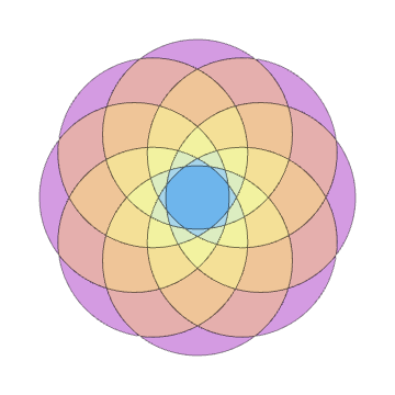
What if we want to color overlapping regions according to how many overlaps they had?

We can use "BooleanCountingFunction" as follows

plots = Table[
   RegionPlot[
    BooleanCountingFunction[{k}, ineqs], {x, -2, 2}, {y, -2, 2}, 
    PlotPoints -> 100, Frame -> None, 
    PlotStyle -> ColorData["Pastel"][k/nc]], {k, 0, nc}];
GraphicsGrid@Partition[plots, 3]
Show[Rest[plots]]

Independence Polynomials with Tree Decomposition

A lot of NP-hard problems on graphs become easy if you find a good tree decomposition of the graph.

Essentially, tree decomposition asks for a way to take a set of small sets of vertices and connect them in a way so that vertices shared by any pair of connected sets is a separator of the graph.

Two examples below show a graph on the left and it's optimal tree decomposition on the right






Following problems become easy once you have a good tree decomposition of a graph. Finding best: clique, independent set, dominating set, TSP tour, Steiner Tree. Almost every graph polynomial is tractable to compute given good tree decomposition. Finding BEST tree decomposition is NP-hard, but finding good decomposition is much easier. It parallelizes well, and simple heuristics give decompositions close to optimal for moderate size graphs even on my two-processor laptop.

Here are two relevant notebooks:

• Compute independence polynomials using tree decomposition
  
• Compute tree decomposition greedily and visualize it

Making Error Correcting code with FindIndependentVertexSet

Suppose you want to transmit information over a lossy channel. Your channel flips some bits at random and you want to choose your code-words so that you can recover the original codeword with high probability.

One approach is to pick a set of codewords of length n so that the Hamming distance between any two of them is at least d. This means that if the number of errors is less than (d-1)/2, you can recover the original word by picking code word closest in Hamming distance to the received word.

For example, for 3 bits and d=2, the code would be

100
010
001
111

Essentially when d=2, this is equivalent to finding a set of non-adjacent vertices of hypercube in n dimensions. For instance, code above can be visually represented as follows



For n=4 we can visualize it as follows


Essentially the problem is one of independent set, we construct a graph where vertices correspond to codewords and are connected if and only if hamming distance between them is 1.

Two graphs above correspond to "CubicalGraph" and "TesseractGraph" in GraphData, but if you want to recover the codewords, you want to control the ordering of vertices and construct the graph yourself. Getting the code is straightforward from the independent vertex set

words = Tuples[{0, 1}, 4];
distMat = Outer[HammingDistance, words, words, 1];
g = AdjacencyGraph[Map[Boole[# == 1] &, distMat, {2}]];
verts = FindIndependentVertexSet[g];
code = words[[verts]]

The result gives you a set of code-words over n-bits that are at least 2 bit flips apart from one another.

Now suppose we want to make our code more robust against errors. We construct graph as before, but augment it with the command "GraphPower[g,d-1]" to create a graph where vertices in an independent set are at least d steps apart. For n=6,d=2, VertexIndependentSet finds a code consisting of 8 codewords, which is the best possible.

It is known that for n=7,d=3 there's a code consisting of 16 codewords, although this problem seems to be too difficult to solve using version of VertexIndependentSet that ships with version 8.0

I'm experimenting with a message passing algorithm to solve this problem in the independent vertex set formulation, I'll post an update if it turns out better than the built-in

Notebook

Magic Square

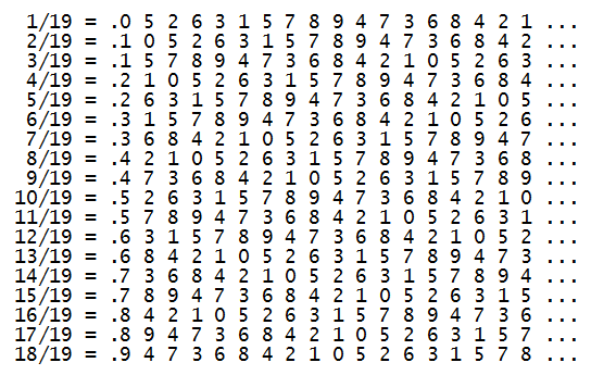
Here's an interesting tidbit I saw linked from reddit -- the following decimal expansions form a magic square



Here's how you'd check the row and column sums

v = 18;
row[k_] := PadLeft[IntegerDigits[Floor[k/(v + 1)*10^v]], v];
mat = row /@ Range[v];
Total@mat
Total@Transpose@mat

Making web animations

I came across this cool animation on Sander Huisman's blog. Original animation was a lossy YouTube link, and it doesn't do it justice. The way to get a high-quality embedded animation is to generate individual frames and then export to Flash format as follows

Export["~/research/qr/hinges/anim.swf", images];

Then include the following snippet in your page. Location of the swf file goes in two places, allegedly to provide compatibility for IE+Mozilla browsers

Notebook